Force-System Resultants and Equilibrium

Study notes on Chapter 1 of The Electrical Engineering Handbook Series — "Force-System Resultants and Equilibrium" (R. C. Hibbeler). Figures are reproduced from the handbook.

Statics studies bodies in equilibrium — at rest or moving at constant velocity. Before applying the equilibrium laws you need two tools: simplifying a force system, and computing the moment of a force.

1.1 Force-system resultants

Concurrent forces

A force is a vector: magnitude, direction, and point of application. Two forces acting through the same point add by the parallelogram law to give a resultant $\mathbf{F}_R = \mathbf{F}_1 + \mathbf{F}_2$.

For more than two forces it is easier to resolve each one into Cartesian components, $\mathbf{F} = F_x\mathbf{i} + F_y\mathbf{j} + F_z\mathbf{k}$, and add component-wise:

$$\mathbf{F}_R = \sum F_x\,\mathbf{i} + \sum F_y\,\mathbf{j} + \sum F_z\,\mathbf{k} \tag{1.1}$$

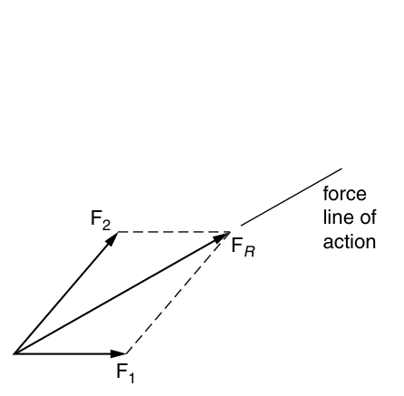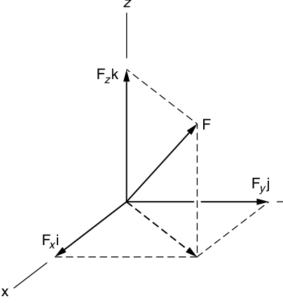Figure 1.1 — Addition of forces by the parallelogram law.	Figure 1.2 — Resolving a vector into x, y, z components.

Moment of a force

Where a force acts matters. Sliding $\mathbf{F}$ along its own line of action (A → B in Figure 1.3) leaves the body's motion unchanged — the principle of transmissibility — though internal stresses differ. Moving it off that line (to C) changes the rotation, because the lines of action are now separated by a distance $d$.

That turning tendency about a point O is the moment:

$$M_O = F d \tag{1.2}$$

where $d$ is the perpendicular distance from O to the line of action. Its direction follows the right-hand rule: curl your fingers with the rotation, and your thumb points along $\mathbf{M}_O$.

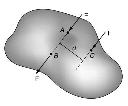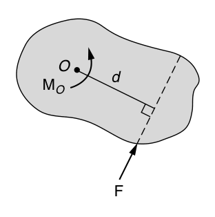Figure 1.3 — Same force at A, B (same line) and C (offset by d).	Figure 1.4 — Moment of a force about O.

When $d$ is awkward to find, use the principle of moments: the moment of a force equals the sum of the moments of its components, so $M_O = F_x y + F_y x$ (Figure 1.5).

In 3D, write it as a cross product, with $\mathbf{r}$ running from O to any point on the line of action:

$$\mathbf{M}_O = \mathbf{r} \times \mathbf{F} \tag{1.3}$$ $$\begin{aligned} \mathbf{M}_O &= \begin{vmatrix} \mathbf{i} & \mathbf{j} & \mathbf{k} \\ x & y & z \\ F_x & F_y & F_z \end{vmatrix} \\ &= (yF_z - zF_y)\,\mathbf{i} + (zF_x - xF_z)\,\mathbf{j} + (xF_y - yF_x)\,\mathbf{k} \end{aligned} \tag{1.4}$$

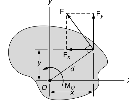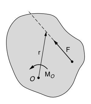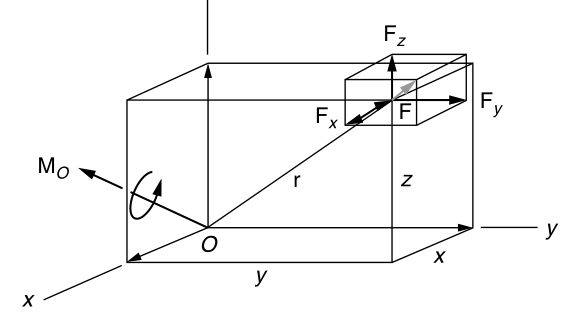Figure 1.5 — Principle of moments.	Figure 1.6 — Moment as r × F.	Figure 1.7 — Cartesian components of the moment.

Couples

A couple is two equal, opposite, parallel forces a distance $d$ apart. Its moment is the same about every point:

$$\mathbf{M}_C = \mathbf{r}_1 \times \mathbf{F} + \mathbf{r}_2 \times (-\mathbf{F}) = (\mathbf{r}_1 - \mathbf{r}_2) \times \mathbf{F} = \mathbf{r} \times \mathbf{F} \tag{1.5}$$

Here $\mathbf{r}$ goes from any point on $-\mathbf{F}$'s line to any point on $\mathbf{F}$'s line. A couple's resultant force is zero, so it rotates a body without translating it.

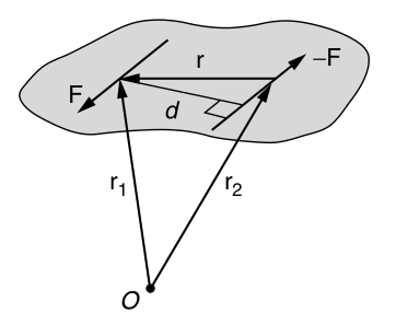
Figure 1.8 — A couple: the moment depends only on the separation r.

Resultant of a force and couple system

Any set of forces and couples can be replaced by one force and one couple moment at a chosen point O:

$$\mathbf{F}_R = \sum \mathbf{F} \tag{1.6}$$ $$\mathbf{M}_{R_O} = \sum \mathbf{M}_O \tag{1.7}$$

$\sum \mathbf{M}_O$ includes $\mathbf{r}_i \times \mathbf{F}_i$ for every force plus every couple moment.

You can go one step further. Split $\mathbf{M}_{R_O}$ into a part parallel to $\mathbf{F}_R$ ($M_\parallel$) and a part perpendicular to it ($M_\perp$). Shifting $\mathbf{F}_R$ sideways by $d = M_\perp / F_R$ absorbs $M_\perp$, leaving a wrench: a force plus a collinear moment — a push and a twist together.

If $\theta = 90^\circ$ then $M_\parallel = 0$ and everything reduces to a single force on a specific line of action. That always happens for concurrent, parallel, or coplanar systems.

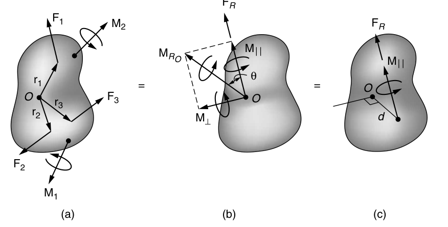
Figure 1.9 — (a) general system → (b) force + couple at O → (c) wrench.

Distributed loadings

Contact loads are really spread over an area. If that area is small, treat it as a point force; if it's large (wind, fluid pressure), describe it with a load-intensity function $p = p(x, y)$. Its resultant and line of action are:

$$F_R = \int_A p(x,y)\,dA \tag{1.8}$$ $$\bar{x} = \frac{\int_A x\,p\,dA}{\int_A p\,dA}, \qquad \bar{y} = \frac{\int_A y\,p\,dA}{\int_A p\,dA} \tag{1.9}$$

Geometrically, $F_R$ is the volume under the load diagram and it acts through that volume's centroid. For a line load $w = w(x)$, $F_R$ is the area under the curve, acting through the area's centroid.

Body forces act through the volume without contact — gravity is the usual one. Its resultant is the weight, acting through the center of gravity.

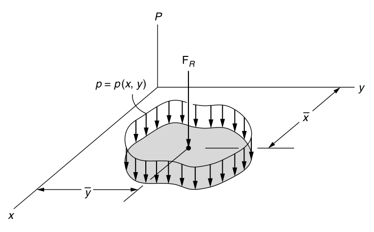
Figure 1.10 — A distributed load p(x, y) and its resultant.

1.2 Equilibrium

Equations of equilibrium

Treat the body as rigid (fine when deformations are small). It is in equilibrium iff the resultant force and moment both vanish:

$$\sum \mathbf{F} = \mathbf{0} \tag{1.10}$$ $$\sum \mathbf{M}_O = \mathbf{0} \tag{1.11}$$

In components that is six scalar equations:

$$\begin{aligned} \sum F_x &= 0, & \sum F_y &= 0, & \sum F_z &= 0 \\ \sum M_x &= 0, & \sum M_y &= 0, & \sum M_z &= 0 \end{aligned} \tag{1.12}$$

Any three non-coplanar, non-parallel axes work for the sums. For a coplanar system only three remain:

$$\sum F_x = 0,\quad \sum F_y = 0,\quad \sum M_O = 0 \tag{1.13}$$

O can be anywhere — on or off the body.

Free-body diagram

Sketch the body isolated ("free") from everything around it and draw every force and couple on it: applied loads, support and contact reactions, and weight. Add the dimensions you'll need for moments. Once the FBD and axes are set, the equilibrium equations are mechanical.

Support reactions

Rule of thumb: a support that blocks translation in a direction exerts a force in that direction; one that blocks rotation exerts a couple moment.

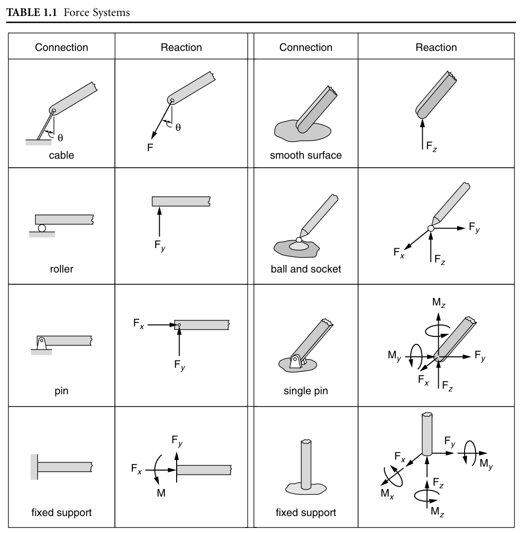
Table 1.1 — Common connections and the reactions they exert.

Friction

A rough surface resists slipping with a force tangent to the surface and opposing the (possible) motion. For dry surfaces:

$$F \le \mu_s N \tag{1.14}$$

Equality holds only when slipping is impending. $N$ is the normal force and $\mu_s$ the coefficient of static friction. Once sliding, $F = \mu_k N$, with $\mu_k$ roughly 25% below $\mu_s$.

Materials	$\mu_s$
Metal on ice	0.03 – 0.05
Wood on wood	0.30 – 0.70
Leather on wood	0.20 – 0.50
Leather on metal	0.30 – 0.60
Aluminum on aluminum	1.10 – 1.70

Table 1.2 — Typical coefficients of static friction.

Constraints

Satisfying the equations is not enough; the body must also be properly held.

• Statically indeterminate — more supports than needed, so more unknowns than equations. The beam in Figure 1.11 has four unknowns ($A_x, A_y, M_A, B_y$) but only three equations; the extra one comes from deformation (mechanics of materials).
• Improperly constrained — the body can move. This happens when the reactions are all parallel (Figure 1.12, nothing resists $\sum F_x$) or all concurrent (Figure 1.13, nothing resists rotation about that point).

If the number of reactions is the minimum and they are neither parallel nor concurrent, the problem is statically determinate.

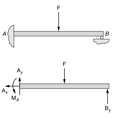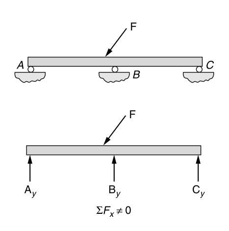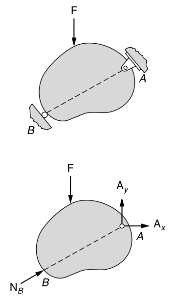Figure 1.11 — Indeterminate beam.	Figure 1.12 — Parallel reactions.	Figure 1.13 — Concurrent reactions.

Internal loadings

The method of sections: if a body is in equilibrium, so is any piece of it. Cut it, draw the FBD of one piece, and the internal resultants become external loads you can solve for.

• In 3D there are six: normal force $N_y$, shears $V_x, V_z$, torque $T_y$, and bending moments $M_x, M_z$ (Figure 1.14).
• For coplanar loads only three: normal force $N$, shear $V$, bending moment $M$ (Figure 1.15).

How those resultants are distributed over the cut (stress) is mechanics of materials.

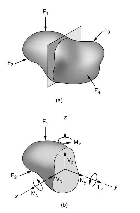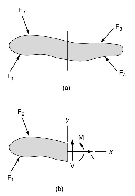Figure 1.14 — Six internal resultants in 3D.	Figure 1.15 — N, V, M for a coplanar load.

Worked examples

The recipe is always the same: pick axes, draw the FBD, apply the equations.

Example 1.1 — Parallel forces on a plate

Reduce the three parallel forces on the plate to one resultant and find where it acts.

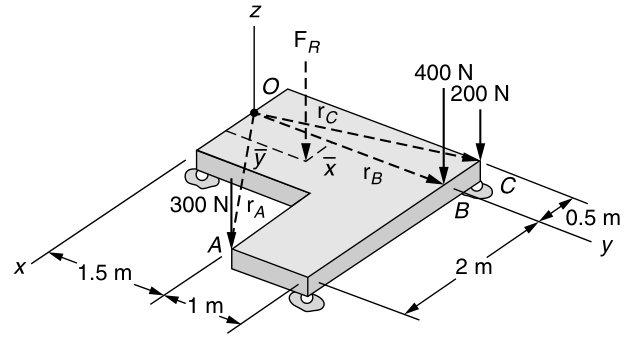
Figure 1.16

$$\mathbf{F}_R = -300\mathbf{k} - 400\mathbf{k} - 200\mathbf{k} = \{-900\mathbf{k}\}\ \text{N}$$ $$\begin{aligned} \mathbf{M}_{R_O} &= (2\mathbf{i}+1.5\mathbf{j})\times(-300\mathbf{k}) + (2.5\mathbf{j})\times(-400\mathbf{k}) + (-0.5\mathbf{i}+2.5\mathbf{j})\times(-200\mathbf{k}) \\ &= \{-1950\mathbf{i} + 500\mathbf{j}\}\ \text{N·m} \end{aligned}$$

As expected for parallel forces, $\mathbf{F}_R \perp \mathbf{M}_{R_O}$. Place $\mathbf{F}_R$ at $(\bar x, \bar y)$ so that $\mathbf{r}\times\mathbf{F}_R = \mathbf{M}_{R_O}$:

$$\bar x = \frac{M_{O_y}}{F_R} = \frac{500}{900} = 0.556\ \text{m}, \qquad \bar y = \frac{M_{O_x}}{F_R} = \frac{1950}{900} = 2.17\ \text{m}$$

Example 1.2 — Beam with a pin and a smooth support

Find the reactions on the beam.

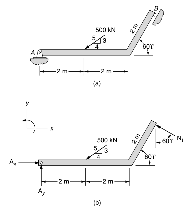
Figure 1.17 — (a) beam, (b) free-body diagram.

From Table 1.1, A is a pin ($A_x, A_y$) and B a smooth contact ($N_B$, normal to the 60° member). Three unknowns, three equations — determinate. Sum moments about A to drop $A_x$ and $A_y$:

$$\begin{aligned} \sum M_A = 0:\quad & -500\left(\tfrac35\right)(2) + N_B\cos 60^\circ\,(4 + 2\cos 60^\circ) \\ & + N_B\sin 60^\circ\,(2\sin 60^\circ) = 0 \;\Rightarrow\; N_B = 150\ \text{N} \end{aligned}$$ $$\sum F_x = 0:\quad A_x - 500\left(\tfrac45\right) - 150\sin 60^\circ = 0 \;\Rightarrow\; A_x = 530\ \text{N}$$ $$\sum F_y = 0:\quad A_y - 500\left(\tfrac35\right) + 150\cos 60^\circ = 0 \;\Rightarrow\; A_y = 225\ \text{N}$$

All positive, so the assumed directions on the FBD are correct. (The figure labels the load "500 kN"; the handbook's solution works in N.)

Example 1.3 — Compound beam

Segments AB and BC are pinned at B. Find the support reactions.

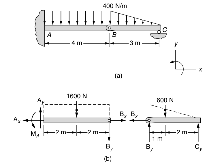
Figure 1.18 — (a) compound beam, (b) FBDs of each segment.

Split at B; by Newton's third law, $B_x$ and $B_y$ act equal and opposite on the two pieces. Replace each distributed load with its resultant: the uniform 400 N/m over 4 m → 1600 N at the midpoint; the triangle over 3 m → $\tfrac12(400)(3) = 600$ N at 1 m from B.

Segment BC:

$$\begin{aligned} \sum F_x = 0&:\quad B_x = 0 \\ \sum M_B = 0&:\quad -600(1) + C_y(3) = 0 \;\Rightarrow\; C_y = 200\ \text{N} \\ \sum F_y = 0&:\quad B_y - 600 + 200 = 0 \;\Rightarrow\; B_y = 400\ \text{N} \end{aligned}$$

Segment AB:

$$\sum F_x = 0:\ A_x = 0 \qquad \sum F_y = 0:\ A_y - 1600 - 400 = 0 \Rightarrow A_y = 2000\ \text{N}$$ $$\sum M_A = 0:\ M_A - 1600(2) - 400(4) = 0 \Rightarrow M_A = 4800\ \text{N·m}$$

Example 1.4 — Table on a rough floor

The table rests on a floor with $\mu_s = 0.3$ and carries 500 N. Find the largest $P$ before it moves.

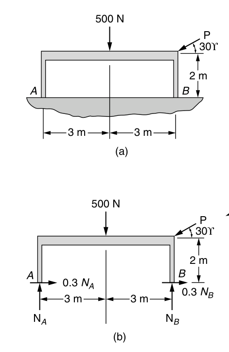
Figure 1.19 — (a) table, (b) free-body diagram with impending slip.

At the maximum, slipping impends at both legs, so $F = 0.3N$ at A and B. Unknowns: $P, N_A, N_B$.

$$\begin{aligned} \sum M_B = 0&:\quad -N_A(6) + 500(3) + P\cos 30^\circ\,(2) = 0 \\ \sum F_x = 0&:\quad 0.3N_A + 0.3N_B - P\cos 30^\circ = 0 \\ \sum F_y = 0&:\quad N_A + N_B - 500 - P\sin 30^\circ = 0 \end{aligned}$$ $$P = 209\ \text{N}, \qquad N_A = 310\ \text{N}, \qquad N_B = 294\ \text{N}$$

Both normal forces are positive, so both legs stay on the floor.

Key terms

• Concurrent forces — forces whose lines of action pass through one point.
• Couple — two equal, opposite, non-collinear forces; produces rotation only.
• Free-body diagram — the body drawn isolated, with every load and needed dimension.
• Friction — tangential resistance one surface exerts on another.
• Method of sections — any cut-out piece of a body in equilibrium is itself in equilibrium.
• Parallelogram law — add two vectors tail-to-tail; the resultant is the parallelogram's diagonal.
• Principle of moments — a force's moment equals the sum of its components' moments.
• Principle of transmissibility — a force may slide along its line of action without changing external effects.
• Weight — Earth's gravitational pull on a body, acting through its center of gravity.
• Wrench — a force plus a collinear moment: a push and a twist.

Reference: Hibbeler, R. C. (2004). Engineering Mechanics: Statics, 10th ed. Prentice Hall.