4.1 Monte Carlo — random numbers

Source: Ideas from Computational Physics (Landau, Páez, Bordeianu), Ch. 4 intro–§4.2. Rewritten in original wording. Continues 3.4b Specular and Bessel labs. Labs: 4.1b Monte Carlo labs.

Deterministic programs are comforting: same input, same output. Yet huge amounts of machine time go into Monte Carlo work — calculations that feed chance-like numbers into a model of a random process (thermal motion, radioactive decay) or into an average that solves an equation. Later chapters reuse the same tools for integration and for thermal / quantum fluctuations. This lesson is the foundation: where those numbers come from, how to spot a bad generator, and what a random walk predicts for diffusion.

4.1 Random numbers

A sequence $r_1,r_2,\ldots$ is random if successive values are uncorrelated. That is not the same as uniform. Uniform means every value in an interval is equally likely ($P(r)=\mathrm{const}$). The integers $1,2,3,\ldots$ are uniform on their lattice and still perfectly predictable. Conversely, a sequence can look “random” while hiding short-range correlations, for example

$$r_1,\ (1-r_1),\ r_2,\ (1-r_2),\ \ldots$$

The usual library generator aims for uniform and uncorrelated draws on $[0,1)$.

Computers are deterministic machines, so they cannot produce true randomness. A computed stream always has a finite period and hidden structure; given enough previous terms you can predict the next. We call the output pseudorandom (and then casually drop the “pseudo”). Better generators hide correlations longer; if you look hard enough, or run long enough, the correlations show. Tables of radioactive counts or hardware noise sources exist as sanity checks, not as production defaults.

Linear congruent (power-residue) method

The classic integer recurrence on $\{0,1,\ldots,M-1\}$ advances a seed $r_1$ by multiply–add–mod, then maps into $[0,1)$. Walk the update, the unit-interval map, and the lattice-rejection rule — pick each equation among lookalikes.

As a tiny walkthrough: $a=4$, $c=1$, $M=9$, $r_1=3$ yields the cycle $3,4,8,6,7,2,0,1,5,3,\ldots$ (length $M=9$). Dividing by $M$ gives $0.333,0.444,0.889,\ldots$. For a general interval $[A,B]$, the affine map $x_i=A+(B-A)r_i$ appears as an optional step in the random-walk guide below.

Large $a$ and $M$ stretch the period (48-bit generators may reach $M\sim 2^{48}$), but overflow and careless constants produce garbage. Prefer an industrial generator (random.random() — Mersenne Twister in CPython) over a homemade LCG for serious work; still plot before you trust.

Quiz

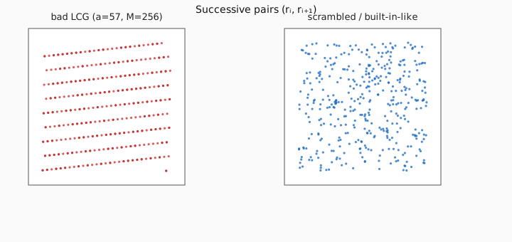
Pseudorandom numbers

1 / 3

Uniform and random are…

Pick an answer to see if you are right.

4.2 Random walk (theory)

A perfume molecule in air takes many collisions before it reaches the back of the room. Model the path as $N$ planar steps $(\Delta x_k,\Delta y_k)$. Expand $R^{2}$, drop averaged cross terms, recover $R_{\mathrm{rms}}\simeq\sqrt{N}\,r_{\mathrm{rms}}$ — pick the matching equation at each step (lookalikes included). An optional last step maps an LCG draw onto $[A,B]$.

Quiz

Random walk

1 / 3

For a random walk with RMS step r_rms, after N steps you expect…

Pick an answer to see if you are right.

Checking the $\sqrt{N}$ law (assessment)

Theory assumed isotropic, uncorrelated steps. After $K$ independent trials,

$$\langle R^{2}(N)\rangle = \frac{1}{K}\sum_{k=1}^{K} R_{(k)}^{2}(N), \qquad R_{\mathrm{rms}} = \sqrt{\langle R^{2}(N)\rangle}.$$

Two diagnostics (the walk above already picked the cross-term and $R_{\mathrm{rms}}^{2}\simeq N r_{\mathrm{rms}}^{2}$ identities):

1. Cross terms near zero on a long single walk and after averaging trials.
2. $R_{\mathrm{rms}}$ vs $\sqrt{N}$. Start at small $N$ (noisy) and push to large $N$ (a few correct digits on average). Different ways of injecting randomness (unit-normalized vs raw box steps) shift the slope but not the $\sqrt{N}$ shape.

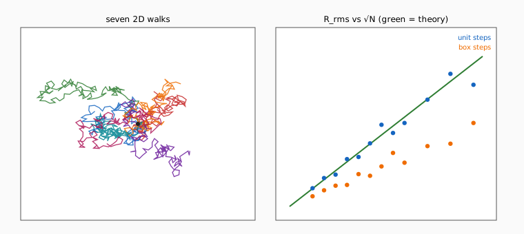
The same averages apply in 3D with unit steps $(\Delta x,\Delta y,\Delta z)$: still $R_{\mathrm{rms}}\simeq\sqrt{N}\, r_{\mathrm{rms}}$, now with three components under the square root.

4.2.2 Random walks in a brain

Understanding a brain is not only neuron wiring — the fluid-filled extracellular spaces between cells shape how drugs, metabolites, and molecular signals diffuse [Nicholson, 2022]. Random-walk models of chemical probes look strikingly like the free walks above. Adding randomly placed circular obstacles (inaccessible pockets) changes the picture: walks that stop or bounce on contact explore less volume, so $R_{\mathrm{rms}}$ drops.

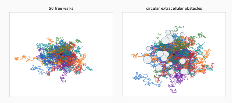
Einstein’s 1905 estimate ties an effective diffusion coefficient to $R_{\mathrm{rms}}$. Walk $D\simeq R_{\mathrm{rms}}^{2}/(2dt)$, the obstructed drop, and the free/obs ratio — pick each equation among lookalikes.

Quiz

Obstructed diffusion

1 / 2

Circular extracellular obstacles typically…

Pick an answer to see if you are right.

4.2.3 Random protein folding (HP model)

A protein chain is a string of monomers: hydrophobic (H) residues prefer to bury away from water; polar (P) residues do not. Folding searches low-energy geometries. Full molecular dynamics is slow; a cheap Monte Carlo cartoon is a self-avoiding random walk on a 2D square lattice [Yue et al., 1995]:

• From the tip, step only to an empty neighbor (three choices at most once the previous site is excluded).
• At each new site, drop an H or P with $P(\mathrm{H})>P(\mathrm{P})$.
• Stop when the tip has no free neighbor (or you hit a length cap).

Energy of a finished chain is $E=-\varepsilon f$ with $f$ counting non-bonded H–H lattice neighbors (P–P and H–P do not help). Compact H cores are the toy “native” states. Walk $E$, $f$, and $\max f\Leftrightarrow\min E$ — pick each equation among lookalikes.

Quiz

HP folding

1 / 3

Self-avoiding means…

Pick an answer to see if you are right.

Next: 4.1b Monte Carlo labs — LCG drills, walk averages, cross terms, brain $R_{\mathrm{rms}}$, HP energy.