4.1b Monte Carlo labs

Source: Lab ideas from Computational Physics (Landau, Páez, Bordeianu), §§4.1.2–4.2.1. Rewritten as original drills. Continues 4.1 Monte Carlo — random numbers.

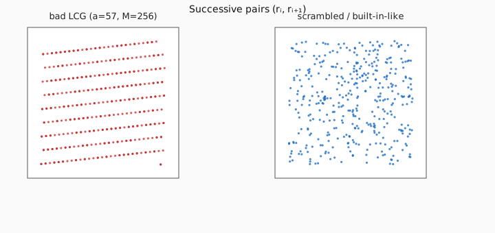
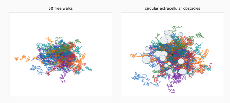
Build a linear congruent generator, measure a pedagogical period, scale into $[A,B]$, then run unit-step 2D walks and compare $R_{\mathrm{rms}}$ to $\sqrt{N}$. Stubs fail until you fill them in. For graded walks we use a fixed LCG as the “random” source so outputs are reproducible.

Formula refresh

Warm up: pick the matching equation among lookalikes (same walk as the theory lesson).

Fixed LCG for graded walks

Build the generator labs with any $(a,c,M)$ from the prompt. For walk labs (4.1b.4 onward), use this shared LCG for draws in $[0,1)$ — not random.random():

# r ← (1103515245 * r + 12345) % 2**31 ; return r / 2**31

Each unit step: draw $\Delta x',\Delta y'$ via $2u-1$ for two uniforms $u$, then normalize to length 1.

Labs

Activity: LCG step

Implement one linear-congruent update: $r\leftarrow (a r + c)\bmod M$.

Input: a c M r. Output: the next integer.

Write-ups

0/8 solved

4.1b.W1

Using “lattice” and “correlation”, explain:

You plot successive pairs $(r_i,r_{i+1})$ from your LCG and see a clear lattice. What does that tell you?

Minimum 3 words. Your answer must include: “lattice”, “correlation”.

0 words/ 3 min

Meet the writing requirements, then you can open the model answer.

Explorers

Reference sketch — random walk

Textbook listings often used VPython (visual) for live plotting. Here is the same idea in plain Python: seed the generator (change the seed for a new path), take steps with independent $\Delta x',\Delta y'\in[-1,1]$, and print the path. For graded labs, use the fixed LCG, not random.random().

# walk_ref.py — 2D random walk (reference sketch)
import random

random.seed(None)  # None => system clock; pass an int for a fixed sequence
N = 20
x = y = 0.0
print(f"{x:.6f} {y:.6f}")
for _ in range(N):
    dx = (random.random() - 0.5) * 2.0  # in [-1, 1]
    dy = (random.random() - 0.5) * 2.0
    # Optional unit step (labs normalize; this sketch matches a raw box step):
    # import math; L = math.hypot(dx, dy) or 1.0; dx, dy = dx / L, dy / L
    x += dx
    y += dy
    print(f"{x:.6f} {y:.6f}")

Reference sketch — self-avoiding HP fold

Textbook demos used VPython for a live grid. Here is the same physics in plain Python: self-avoiding steps on the square lattice, H more often than P, stop when the tip is boxed in, score $E=-\varepsilon f$ from non-bonded H–H contacts (the old “yellow dots”).

# protein_fold_ref.py — self-avoiding HP walk (reference sketch)
import random

DIRS = [(1, 0), (-1, 0), (0, 1), (0, -1)]

def select_hp(p_h=0.7):
    return "H" if random.random() <= p_h else "P"

def fold(max_len=40, p_h=0.7, seed=None):
    random.seed(seed)
    occ = {(0, 0)}
    chain = [(0, 0, select_hp(p_h))]
    while len(chain) < max_len:
        x, y, _ = chain[-1]
        free = [(x + dx, y + dy) for dx, dy in DIRS if (x + dx, y + dy) not in occ]
        if not free:
            break  # corner / occupied neighbors — stop
        nx, ny = random.choice(free)
        occ.add((nx, ny))
        chain.append((nx, ny, select_hp(p_h)))
    return chain

def energy(chain, eps=1.0):
    index = {(x, y): i for i, (x, y, _) in enumerate(chain)}
    f = 0
    seen = set()
    for i, (x, y, kind) in enumerate(chain):
        if kind != "H":
            continue
        for dx, dy in DIRS:
            j = index.get((x + dx, y + dy))
            if j is None or j <= i or abs(i - j) == 1:
                continue
            if chain[j][2] != "H":
                continue
            if (i, j) in seen:
                continue
            seen.add((i, j))
            f += 1
    return -eps * f, f

if __name__ == "__main__":
    chain = fold(max_len=36, seed=11)
    E, f = energy(chain)
    print("length", len(chain), "f", f, "E", E)
    for x, y, k in chain:
        print(x, y, k)

Next: 4.2 Spontaneous decay.