4.2 Spontaneous decay

Source: Ideas from Computational Physics (Landau, Páez, Bordeianu), §4.3. Rewritten in original wording. Continues 4.1b Monte Carlo labs. Labs: 4.2b Spontaneous decay labs.

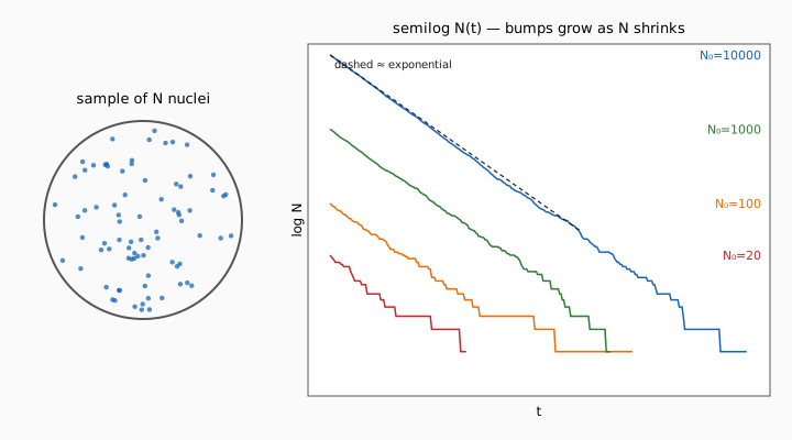
Simulate a small sample of $N$ radioactive nuclei and watch how stochastic decay relates to the familiar exponential law. Exponential decay is an excellent continuum model when $N$ is huge; it is only an approximation once few particles remain. A discrete Monte Carlo decay — each surviving nucleus flips a coin each $\Delta t$ — is closer to a Geiger counter: random clicks whose average rate falls as the sample empties (Figure 4.7).

Spontaneous decay needs no external kick. The probability that any one nucleus decays in a unit time interval is a constant $\lambda$, independent of age and of how many neighbors are left. When it decays, it is gone. The activity (decays per $\Delta t$) therefore falls as $N$ falls, even though each survivor still faces the same $\lambda$.

Discrete decay model

Let $N(t)$ be the number still present and $\Delta N(t)$ the number that decay in a short $\Delta t$. Walk $\mathcal{P}=-\lambda$, the finite-difference activity law, the continuum ODE, and the exponential solution — pick the matching equation at each step.

This is a finite-difference relation among measurable quantities. It cannot be integrated like a DE, but it can be simulated: $\Delta N$ in any one step is random; the average over many identical samples is predictable.

Exponential as a large-$N$ limit

Exponential decay is the mean-field description when $N\to\infty$ and $\Delta t\to 0$ (the guide’s last two steps). Nature often has small $N$; then the discrete hazard still holds particle-by-particle, but the exponential becomes a smooth envelope, not the path of a single sample.

Activity in the continuum limit:

$$\frac{dN}{dt}(t)=-\lambda N(0)e^{-\lambda t}.$$

Discrete simulation

Advance time in steps of $\Delta t$. For each step, loop over the nuclei that remain; each decays independently if a uniform random $r_i<\lambda$ (with $\lambda$ measured in units of $1/\Delta t$). Stop when $N=0$:

input N, λ
t ← 0
while N > 0
    Δ ← 0
    for each of the N nuclei
        if r_i < λ then Δ ← Δ + 1
    t ← t + 1
    N ← N − Δ
    output t, Δ, N

Choosing $\lambda$ sets the time unit. If a physical rate is $0.3\times 10^{6}\,\mathrm{s}^{-1}$ and you tick in microseconds, use $\lambda\simeq 0.3$ with $r\in[0,1]$. For qualitative slopes you can ignore absolute units and focus on $-\lambda$ on a semilog plot.

Quiz

Spontaneous decay

1 / 4

The microscopic statement “each nucleus has constant decay probability per unit time” is written…

Pick an answer to see if you are right.

Why randomness yields an exponential envelope. Each survivor faces the same hazard $\lambda$. The expected change is $\langle\Delta N\rangle=-\lambda N\Delta t$, which is exactly the continuum law. Fluctuations of order $\sqrt{N}$ (roughly) become invisible on a plot when $N$ is $10^5$ and scream when $N$ is $20$ — same law, different sample size.

Not a power law. A pure $N=\beta t^{-\alpha}$ is a straight line on log–log axes, not on semilog. Stochastic exponential stays near a straight semilog line while $N$ is large; a power-law fit to the same window has larger residuals (labs).

Next: 4.2b Spontaneous decay labs.